Getting started¶

A quick overview of FLEXPART data¶

pflexible was originally developed for working with FLEXPART V8.x which has some fairly new features to how the output data is created. The latest version of FLEXPART also has functionality for saving directly to Netcdf. The ability to read this data directly is forthcoming, but for now pflexible still only works with the raw unformatted binary Fortran data FLEXPART has traditionally used for output. See the documents for information regarding FLEXPART .

A users guide for FLEXPART is available which explains the model output.

Note If you are interested in contributing functionality for other FLEXPART versions, please contact me.

pflexible was originally released as ‘pflexpart’, but as the goal is to be more generic, the package was renamed. The current release is still focused on FLEXPART, but some generalizations are starting to make their way into the code base.

pflexible is undergoing constant modifications and is not particularly stable or backward compatible code. I am trying to move in the right direction, and have moved the code now to bitbucket.org. If you are interested in contributing, feel free to contact me: John F. Burkhart

Fetching example data¶

An example data set is available for testing. The data contains a simple backward run case, and thus is suitable for testing some of the unique functions of pflexible for analysis and creation of the retroplumes.

I suggest using wget to grab the data:

wget http://folk.uio.no/johnbur/sharing/flexpart_V8data.tgz

Testing pflexible¶

Once you have checked out the code and have a sufficient FLEXPART dataset to work with you can begin to use the module. The first step is to load the module. Depending on how you checked out the code, you can accomplish this in a few different way, but the preferred is as follows:

import pflexible as pf

The next step is to read the FLEXPART header file from a dataset:

H = pf.Header('/path/to/flexpart/output')

Now you have a variable ‘H’ which has all the information about the run that is available from the header file. This ‘Header’ is essentially a dictionary, so the first step may be to explore some of the keys:

H.keys()

This should produce some output that looks familiar to your from your FLEXPART run setup.

Reasonably, you should now want to read in some of the data from your run. This is accomplished easily using the read_grid. This function may be called directly, or there are several alternative ways we can read the data. A special method exists for backward runs that collects all the data from the 20-days back in time (by default) and creates accumulated totals of the sensitivity:

H.fill_backwards()

Alternatively, we may only want to read specific grids, in which case we can call the function directly:

FD = pf.read_grid(H,time_ret=0,nspec_ret=0)

For optimal performance, this function will use the FortFlex module. However, as a fall back there is a pure python method, but it is significantly slower. If you receive a message about using the Pure Python approach it is highly recommended to build the FortFlex module. If you are having problems compiling FortFlex, see the section in the Installation instructions.

Note

See the read_grid function for information on the keyword arguments.

At this point you should now have a variable ‘FD’ which is again a dictionary of the FLEXPART grids. This ‘FD’ object is either available directly in your workspace, or alternatively, if you called H.fill_backward() it is an attribute of the header: H.FD. This is the preferred method.

Look at the keys of the dictionary to see what information is stored. The actual data is keyed by tuples: (nspec, datestr) where nspec is the species number and datestr is a YYYYMMDDHHMMSS string for the grid timestep.

Working with pf... in depth¶

Assuming the above steps worked out, then we can proceed to play with the tools in a bit more detail.

Okay, let’s take a look at the example code above line by line. The first line imports the module, giving it a namespace “pf” – this is the preferred approach. The next few lines simply define the paths for “SOURCE_DIR” and “OUTPUT_DIR” (you probably already changed these).:

import pflexible as pf

The next line creates a Header class “H”, by passing the path of the directory (not header path) containing the FLEXPART run.:

H = pf.Header(SOURCE_DIR)

The Header is central to pflexible. This contains much information about the FLEXPART run, and enable plotting, labeling of plots, looking up dates of runs, coordinates for mapping, etc. All this information is contained in the Header. See for example:

dir(H)

This will show you all the attributes associated with the Header.

Note

This example uses the methods of the Header class, plexpart.Header. You can also call most the methods directly, passing “H” as the first argument as in: D = pf.fill_backward(H). In some cases, for some of the functions, H can be substituted. See the docstrings for more information.

H is now an object in your workspace. Using Ipython you can explore the methods and attributes of H. As mentioned above, in this test case we call the fill_backward method to populate the “FD” attribute (a dictionary) with all the data from the run.:

H.fill_backward(nspec=(0,1))

However, note that fill_backward also creates a second dictionary attribute “C”. This dictionary is similar to the “FD” dictionary, but contains the Cumulative sensitivity at each time step, so you can use it for plotting retroplumes.

It is important to understand the differences between H.FD and H.C while working with pflexible. If we look closely at the keys of H.FD:

In [13]: H.FD.keys()
Out[13]:
[(0, '20100527210000'),
(0, '20100513210000'),
(0, '20100528210000'),
(0, '20100526210000'),
(0, '20100521210000'),
'grid_dates',
(0, '20100512210000'),
(0, '20100514210000'),
(0, '20100519210000'),
(0, '20100520210000'),
'options',
(0, '20100523210000'),
(0, '20100525210000'),
(0, '20100530210000'),
(0, '20100515210000'),
(0, '20100531210000'),
(0, '20100517210000'),
(0, '20100529210000'),
(0, '20100524210000'),
(0, '20100516210000'),
(0, '20100522210000'),
(0, '20100518210000')]

You’ll see that along with the keys, grid_dates and options, the dictionary is primary keyed by a set of tuples. These tuples represent (s, date), where s is the specied ID and date is the date of a grid file from flexpart (e.g. something like: grid_time_20100515210000_001). However, if we look at the keys of the H.C dictionary:

In [14]: H.C.keys()
Out[14]: [(0, 1), (0, 0), (0, 6), (0, 5), (0, 4), (0, 3), (0, 2)]

We see only tuples, now keyed by (s,rel_id), where s is still the species ID, but rel_id is the release ID. These release IDs correspond to the times in H.releasetimes which is a list of the release times.

Each tuple is a key to another dictionary, that contains the data. Currently there are differences between the way the data is stored in H.FD and in H.C, but future versions are working to make these two data stores common.

So we know now H.C is keyed by (s,k) where s is an integer for the species #, and k is an integer for the release id. Let’s look at the data stores returned in each of these two dictionaries:

In [30]: H.FD[(0, '20100527210000')].keys()
Out[30]:
['dry',
'itime',
'min',
'max',
'gridfile',
'wet',
'rel_i',
'shape',
'spec_i',
'grid',
'timestamp',
'species']

If we look at H.FD[(0, ‘20100527210000’)].grid for example, we’ll see that this returns a numpy array of shape:

In [31]: H.FD[(0, '20100527210000')].grid.shape
Out[31]: (720, 180, 3, 7)

which corresponds to (numx, numy, numz, numk) where numk is the number of releases. We can see this grid is from the gridfile:

In [32]: H.FD[(0, '20100527210000')].gridfile
Out[32]:
'/home/johnbur/Dev_fp/test_data/grid_time_20100527210000_001'

The other information is mainly metadata for that grid.

In H.C the information is slightly different:

In [33]: H.C[(0,1)].keys()
Out[33]:
['itime',
'min',
'timestamp',
'gridfile',
'rel_i',
'shape',
'spec_i',
'grid',
'max',
'species',
'slabs']

In particular, note the shape of the grid is now:

In [35]: H.C[(0,1)].grid.shape
Out[35]: (720, 180, 3)

There is no longer a fourth dimension corresponding to the release time. Furthermore, there is a new key slabs. This is a dictionary where each numz level is packaged as a 2-d numpy array keyed by it’s level index. This is redundant data to the grid, and will likely change in future versions of pflexible. However, the important point to note is that the 0th element is the Total Column.

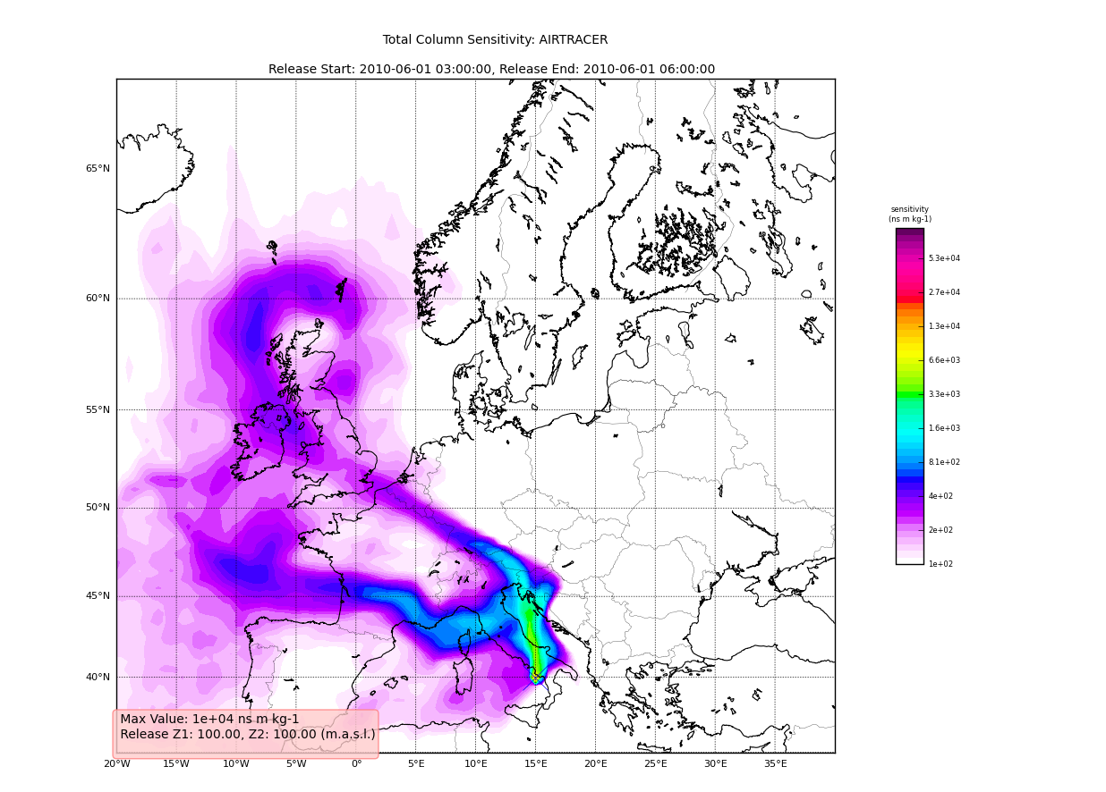
Using the plotting tools of pflexible we can plot the total column easily:

pf.plot_totalcolumn (H, H.C[(0,1)], map_region='Europe')

This should return an image similar to:

Adding Trajectories¶

I use the read_trajectories() function to read the trajectories.txt file and get the trajectories from the run output directory.:

T = pf.read_trajectories(H)

Note, that the only required parameter is the Header “H”, this provides all the metadata for the function to read the trajectories. This is a function that accepts simply the “H” instance or a path to a trajectories file.

Now we can see how we might batch process a backward run and create total column plots as well as add the trajectory information to the plots. The following lines plot the data sets using the plot_totalcolumn(), plot_trajectory(), and plot_footprint().

Warning

There is a lot of reliance on the mapping module in the plot_routines. If you have problems, see the mapping.py file. Or the mapping docstrings. Documentation of this module is presently incomplete but I am working on it.

In order to reuse figures which is much faster when working with the basemap module, I create a “None” objects for passing the figure instances around:

TC = None

After that we loop over the keys (s=species, and k=rel_i) of the H.C attribute we created by calling fill_backward. Note, I named this attribute C for “Cumulative”. In each iteration, for a new combination of s,k we pull the data object out of the dictionary. The “data” object is returned from the function readgridV8() and has some attributes that we can use later in conjunction with the plot_totalcolumn() function and for saving and naming the figures. See for example the following lines:

for s,k in H.C:
    data = H.C[(s,k)]
    TC = pf.plot_totalcolumn(H,data,map_region='Europe',FIGURE=TC)
    TC = pf.plot_trajectory(H,T,k,FIGURE=TC)
    filename = '%s_tc_%s.png' % (data.species, data.timestamp)
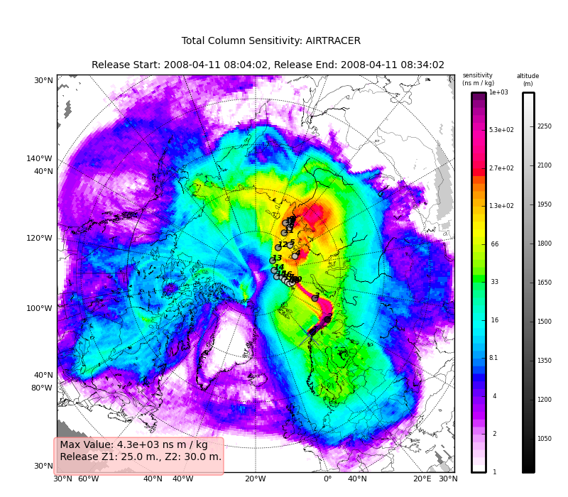
    TC.fig.savefig(filename)

This will create filenames based on the data metadata and save the figure to the path defined by filename. You should now have several images looking like this:

The next step is the use the source and learn more about the functionality of the module. I highly recommend the Ipython interpreter and use of the Tab key to explore the modules methods.

Enjoy!